This page was generated from /home/docs/checkouts/readthedocs.org/user_builds/xdesign/checkouts/0.5.x/docs/source/demos/NoReferenceMetrics.ipynb.
Interactive online version:
![]()
No Reference Metrics
Demonstrate the use of the no-reference metrics: noise power spectrum (NPS), modulation transfer function (MTF), and noise equivalent quanta (NEQ).
[1]:
import matplotlib.pylab as plt
import numpy as np
import tomopy

from xdesign import *
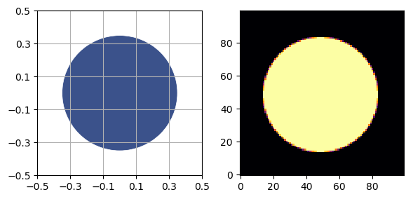
Simulate data aqcuisition
Generate a UnitCircle standards phantom. For the modulation transfer function (MTF), the radius must be less than 0.5, otherwise the circle touches the edges of the field of view.
[2]:
NPIXEL = 100
[3]:
p = UnitCircle(radius=0.35, material=SimpleMaterial(7.23))
sidebyside(p, NPIXEL)
plt.show()
Noise power spectrum (NPS) and Noise Equivalent Quanta (NEQ) are meaningless without noise, so add some poisson noise to the simulated data using np.random.poisson. Collecting two sinograms allows us to isolate the noise by subtracting out the circle.
[4]:
# Define the scan positions using theta and horizontal coordinates
theta, h = np.meshgrid(np.linspace(0, np.pi, NPIXEL, endpoint=False),
                       np.linspace(0, 1, NPIXEL, endpoint=False) - 0.5 + 1/NPIXEL/2)
# Reshape the returned arrays into vectors
theta = theta.flatten()
h = h.flatten()
[5]:
num_photons = 1e4
# Define a probe that sends 1e4 photons per exposure
probe = Probe(size=1/NPIXEL, intensity=num_photons)
# Measure the phantom
data = probe.measure(p, theta, h)
/home/beams0/DCHING/Documents/xdesign/src/xdesign/geometry/algorithms.py:54: RuntimeWarning: halfspacecirc was out of bounds, -1.1249850495609337e-09
  RuntimeWarning)
/home/beams0/DCHING/Documents/xdesign/src/xdesign/geometry/algorithms.py:54: RuntimeWarning: halfspacecirc was out of bounds, -1.597134646758036e-10
  RuntimeWarning)
/home/beams0/DCHING/Documents/xdesign/src/xdesign/geometry/algorithms.py:54: RuntimeWarning: halfspacecirc was out of bounds, -7.460398965264403e-11
  RuntimeWarning)
/home/beams0/DCHING/Documents/xdesign/src/xdesign/geometry/algorithms.py:54: RuntimeWarning: halfspacecirc was out of bounds, -8.34076696598629e-11
  RuntimeWarning)
/home/beams0/DCHING/Documents/xdesign/src/xdesign/geometry/algorithms.py:54: RuntimeWarning: halfspacecirc was out of bounds, -1.9854995425561128e-10
  RuntimeWarning)
[6]:
# Add poisson noise to the result.
noisy_data_0 = np.random.poisson(data)
noisy_data_1 = np.random.poisson(data)
# Normalize the data by the incident intensity
normalized_data_0 = noisy_data_0 / num_photons
normalized_data_1 = noisy_data_1 / num_photons
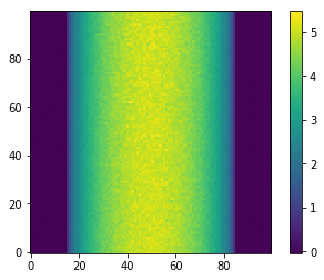
[7]:
# Linearize the data by taking the negative log
sinoA = -np.log(normalized_data_0).reshape(NPIXEL, NPIXEL).T
sinoB = -np.log(normalized_data_1).reshape(NPIXEL, NPIXEL).T
[8]:
plt.imshow(sinoA, cmap='viridis', origin='lower')
plt.colorbar()
plt.show()
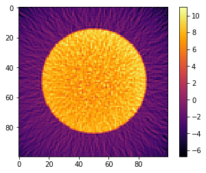
[9]:
# Reconstruct the data using TomoPy
recA = tomopy.recon(np.expand_dims(sinoA, 1), theta,
                    algorithm='gridrec', center=(sinoA.shape[1]-1)/2.) * NPIXEL
recB = tomopy.recon(np.expand_dims(sinoB, 1), theta,
                    algorithm='gridrec', center=(sinoB.shape[1]-1)/2.) * NPIXEL
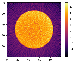
[10]:
plt.imshow(recA[0], cmap='inferno', interpolation="none")
plt.colorbar()
plt.savefig('UnitCircle_noise0.png', dpi=600,
        orientation='landscape', papertype=None, format=None,
        transparent=True, bbox_inches='tight', pad_inches=0.0,
        frameon=False)
plt.show()
[11]:
plt.imshow(recB[0], cmap='inferno', interpolation="none")
plt.colorbar()
plt.show()
Calculate MTF
Friedman’s method
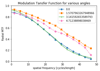
Use Friedman et al’s method for computing the MTF. You can separate the MTF into multiple directions or average them all together using the Ntheta argument.
[12]:
mtf_freq, mtf_value, labels = compute_mtf_ffst(p, recA[0], Ntheta=4)
The MTF is really a symmetric function around zero frequency, so usually people just show the positive portion. Sometimes, there is a peak at the higher spatial frequencies instead of the MTF approaching zero. This is probably because of aliasing noise content with frequencies higher than the Nyquist frequency.
[13]:
plot_mtf(mtf_freq, mtf_value, labels)
plt.gca().set_xlim([0,50]) # hide negative portion of MTF
plt.show()
Siemens star method
You can also use a Siemens Star to calculate the MTF using a fitted sinusoidal method instead of the slanted edges that the above method uses.
[14]:
s = SiemensStar(n_sectors=32, center=Point([0, 0]), radius=0.5)
d = sidebyside(s, 100)
plt.show()
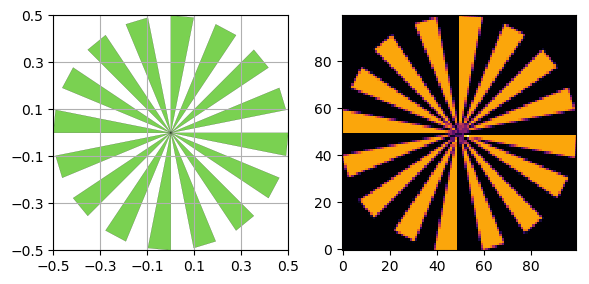
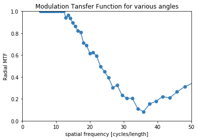
Here we are using the discreet verison of the phantom (without noise), so we are only limited by the resolution of the image.
[15]:
mtf_freq, mtf_value = compute_mtf_lwkj(s, d)
[16]:
plot_mtf(mtf_freq, mtf_value, labels=None)
plt.gca().set_xlim([0,50]) # hide portion of MTF beyond Nyquist frequency
plt.show()
Calculate NPS
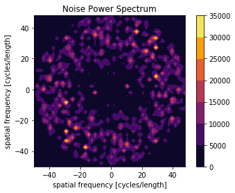
Calculate the radial or 2D frequency plot of the NPS.
[17]:
X, Y, NPS = compute_nps_ffst(p, recA[0], plot_type='frequency',B=recB[0])
[18]:
plot_nps(X, Y, NPS)
plt.show()
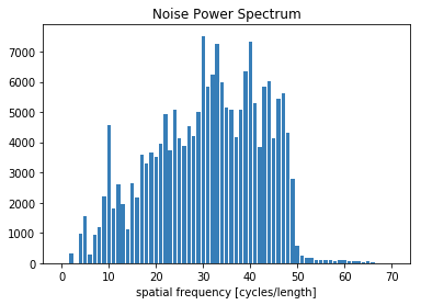
[19]:
bins, counts = compute_nps_ffst(p, recA[0], plot_type='histogram',B=recB[0])
[20]:
plt.figure()
plt.bar(bins, counts)
plt.xlabel('spatial frequency [cycles/length]')
plt.title('Noise Power Spectrum')
plt.show()
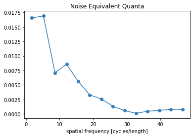
Calculate NEQ
[21]:
freq, NEQ = compute_neq_d(p, recA[0], recB[0])
[22]:
plt.figure()
plt.plot(freq.flatten(), NEQ.flatten())
plt.xlabel('spatial frequency [cycles/length]')
plt.title('Noise Equivalent Quanta')
plt.show()